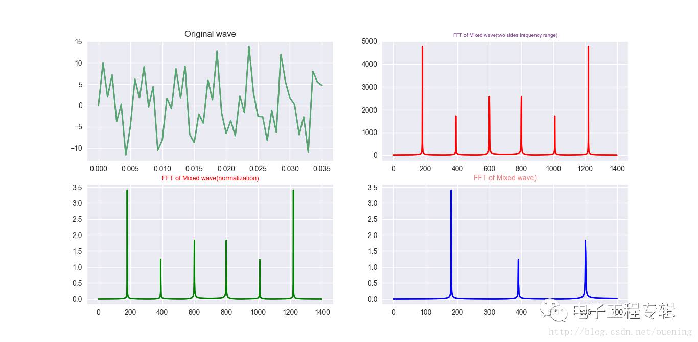
Here is a record of the Fast Fourier Transform (FFT) process. I won't go into detailed explanations about FFT, but instead, I'll provide the code with comprehensive comments for clarity: Import necessary libraries: Set up the sampling parameters. We choose 1400 sampling points because the highest frequency in the signal is 600 Hz. According to the Nyquist sampling theorem, the sampling frequency must be more than twice the highest frequency, so we set it to 1400 Hz: Define the signal composed of three sine waves with frequencies 180 Hz, 390 Hz, and 600 Hz: Perform the FFT and extract real and imaginary parts: Compute the absolute value of the FFT result and normalize it by the number of samples: Due to the symmetry of the FFT output, we only take the first half of the spectrum for plotting: Plot the original signal and its FFT results in different formats: Here's a simple example to further illustrate the FFT process: Niobium Alloys,Niobium Sheet Stock,Tantalum Niobium Alloys,Tantalum Niobium Alloy Customization Shaanxi Xinlong Metal Electro-mechanical Co., Ltd. , https://www.cnxlalloys.comimport numpy as np
from scipy.fftpack import fft, ifft
import matplotlib.pyplot as plt
import seaborn
x = np.linspace(0, 1, 1400)
y = 7 * np.sin(2 * np.pi * 180 * x) + 2.8 * np.sin(2 * np.pi * 390 * x) + 5.1 * np.sin(2 * np.pi * 600 * x)
yy = fft(y)
yreal = yy.real
yimag = yy.imag
yf = abs(fft(y))
yf1 = abs(fft(y)) / len(x)
yf2 = yf1[range(int(len(x)/2))]
xf = np.arange(len(y))
xf1 = xf
xf2 = xf[range(int(len(x)/2))]
plt.subplot(221)
plt.plot(x[0:50], y[0:50])
plt.title('Original Wave')

plt.subplot(222)
plt.plot(xf, yf, 'r')
plt.title('FFT of Mixed Wave (Two Sides Frequency Range)', fontsize=7, color='#7A378B')

plt.subplot(223)
plt.plot(xf1, yf1, 'g')
plt.title('FFT of Mixed Wave (Normalization)', fontsize=9, color='r')

plt.subplot(224)
plt.plot(xf2, yf2, 'b')
plt.title('FFT of Mixed Wave', fontsize=10, color='#F08080')
plt.show()
# -*- coding: utf-8 -*-
import matplotlib.pyplot as plt
import numpy as np
import seaborn
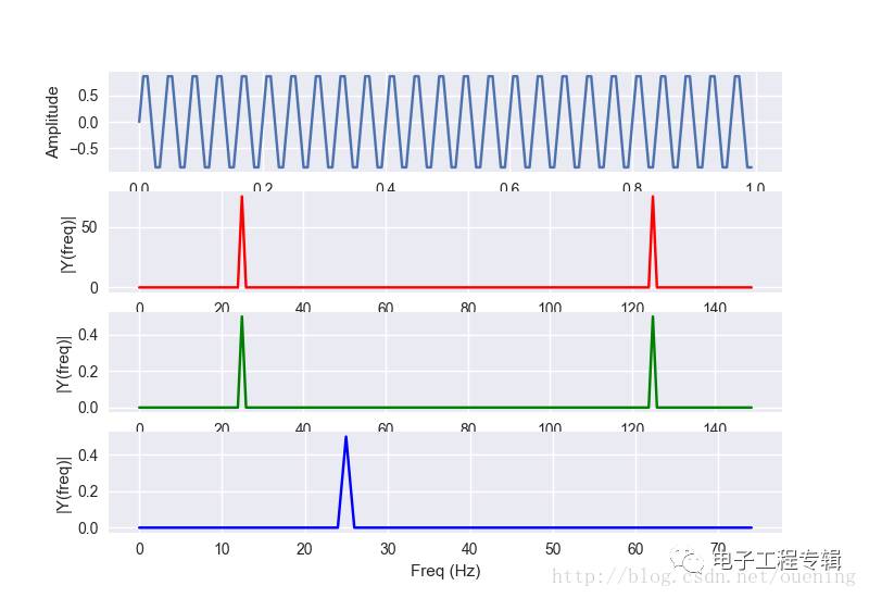
Fs = 150.0 # Sampling rate
Ts = 1.0 / Fs # Sampling interval
t = np.arange(0, 1, Ts) # Time vector
ff = 25 # Frequency of the signal
y = np.sin(2 * np.pi * ff * t)
n = len(y) # Length of the signal
k = np.arange(n)
T = n / Fs
frq = k / T # Two sides frequency range
frq1 = frq[range(int(n / 2))] # One side frequency range
YY = np.fft.fft(y) # FFT without normalization
Y = np.fft.fft(y) / n # FFT with normalization
Y1 = Y[range(int(n / 2))]
fig, ax = plt.subplots(4, 1)
ax[0].plot(t, y)
ax[0].set_xlabel('Time')
ax[0].set_ylabel('Amplitude')
ax[1].plot(frq, abs(YY), 'r') # Plotting the spectrum
ax[1].set_xlabel('Freq (Hz)')
ax[1].set_ylabel('|Y(freq)|')
ax[2].plot(frq, abs(Y), 'g') # Plotting the normalized spectrum
ax[2].set_xlabel('Freq (Hz)')
ax[2].set_ylabel('|Y(freq)|')
ax[3].plot(frq1, abs(Y1), 'b') # Plotting the one-sided spectrum
ax[3].set_xlabel('Freq (Hz)')
ax[3].set_ylabel('|Y(freq)|')
plt.show()